This is the sixth chapter of the tutorial series: Implement a RecSys.
- Chapter 1: Introduction and Project Overview
- Chapter 2: Understanding the Data and Feature Engineering
- Chapter 3: Negative Sampling
- Chapter 4: Offline Evaluation, MLflow Experiment Tracking, and Baseline Implementation
- Chapter 5: Design Session-based Recommendation System
- Chapter 6: Preparing for Serving
- Chapter 7: Building the API Layer
Introduction
In Chapter 5, we have come a long way to build our sequence-based recommendation model which demonstrates significant metric uplifts over the popularity baseline. We also discuss some design decisions regarding the retrieval architecture and how to make it efficient at serving time.
We’re finally ready to tell the world about our exciting new model! To do that, we need to package our work in a way that end-users can benefit from.
This chapter aims to provide a transition ground from model development to deployment readiness. The goal is for us to understand what’s required from model serving point of view, as well as the set ups needed to get it ready.
Deploying ML models in production is actually a very huge area and deserves a series of its own. Within the scope of this tutorial, we will discuss the topic from the angle of an end-to-end data scientist—whose job is to design the complete pipeline from training to serving.
All code for this chapter is available in the notebooks/020-ann-index.ipynb and notebooks/021-store-user-item-sequence.ipynb files, along with the infrastructure configuration in compose.yml and the mlflow/ directory in the project repository.
Serving Paradigms: From Model to User Experience
I have been always thinking that building a recommendation model is like crafting a perfect recipe for a gourmet dish. You might have the most sophisticated ingredients, precise measurements, and innovative techniques, but until that dish reaches hungry customers, it’s just potential sitting in the kitchen. The recipe itself doesn’t feed anyone—it’s the execution, plating, and delivery that creates value. Similarly, our sequence-based recommendation model, no matter how accurate its predictions, remains useless until it can respond to real user requests in real-time.
This analogy extends further when we consider the restaurant’s serving strategy. A restaurant doesn’t prepare each dish from scratch when a customer orders. Instead, they use a combination of pre-preparation (mise en place) and real-time cooking. Some components are prepped in batches during quiet hours, while others must be prepared fresh to order. Recommendation systems follow the same principle: we balance pre-computed results with real-time inference based on the specific requirements of each use case.
How Recommendations Reach Users
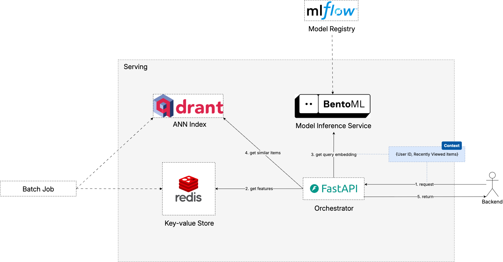
Understanding serving paradigms starts with tracing the journey from user action to displayed recommendations. When a user opens your app, a carefully orchestrated process begins:
- Frontend Request: The mobile app or web interface detects the user’s need for recommendations (homepage load, category browse, search query)
- API Call: The frontend makes a REST API call to the backend, passing user context (user ID, current page, device info)
- Backend Processing: The recommendation service processes this request, either by looking up pre-computed results or fetching the other features necessary for the model to make inference
- Response Assembly: Results are ranked, filtered for business rules, and formatted for display
- Frontend Rendering: The app receives the recommendations and renders them in the user interface
While the actual requirements vary between use cases, normally this entire pipeline must complete within 200ms at the 95th percentile to maintain user engagement. Any longer, and users start experiencing the dreaded loading spinner that kills conversion rates.
Two Paradigms: Batch Pre-computation vs Online Serving
The critical decision in this pipeline happens at step 3: how does the backend generate recommendations? There are two fundamental paradigms, each with distinct trade-offs:
Batch Pre-computation follows the “prepare ahead” strategy. Recommendations are generated offline for all users during low-traffic periods and stored in a key-value store like Redis or DynamoDB. When a user makes a request, the API simply looks up their pre-computed recommendations—a blazingly fast operation that typically completes in under 10ms.
# Batch pre-computation approach
def batch_generate_recommendations():
    """Run offline to pre-compute recommendations for all users."""
    for user_id in all_users:
        recommendations = model.predict(user_id)
        redis_client.set(f"recs:{user_id}", recommendations, ex=3600)

def serve_recommendations(user_id):
    """Fast lookup during serving."""
    return redis_client.get(f"recs:{user_id}")
Online Serving follows the “cook to order” strategy. The model inference happens in real-time when users make requests. This requires the recommendation model to be deployed as a service that can respond to API calls within milliseconds.
# Online serving approach
def serve_recommendations(user_id, context):
    """Real-time model inference during serving."""
    user_features = get_user_features(user_id)
    contextual_features = extract_context(context)
    return model.predict(user_features, contextual_features)
When to Choose Each Paradigm
The choice between batch pre-computation and online serving isn’t arbitrary—it depends on your specific constraints and requirements. Batch pre-computation shines when recommendations don’t need real-time context. It’s also ideal when you can tolerate slightly stale recommendations that are updated periodically, perhaps hourly or daily, in exchange for guaranteed fast response times under all conditions. And it’s particularly attractive when your infrastructure needs to be simple and cost-effective, especially if you’re serving millions of users and want predictable resource utilization patterns.
On the other hand, online serving becomes essential when having access to real-time contexts for recommendations is crucial in ensuring the relevance of our recommendations. Those contexts can be a user’s current shopping cart contents, her search query, or time-sensitive factors like current location or weather. All of these signals share an important property: we don’t know them in advance, so pre-computation is not an option.
In practice, most production recommendation systems use a hybrid approach that combines both paradigms strategically. The default fallback homepage might display pre-computed “trending items” in cases of new users or errors from the recommendation services. In the remaining happy cases, we pass the relevant contexts to the model endpoints to provide better browsing experiences for users. This hybrid strategy optimizes for both performance and personalization.
As you can see, the UI demo for our project also starts by showing the popular recommendations before updating the list with respect to user’s interactions.
Three-Pillar Serving Architecture
How to implement this hybrid serving strategy?
We’ll set up three main components that form the backbone of serving our retrieval model: MLflow for model registry and deployment, Qdrant for vector similarity search, and Redis as KV store for user sequences and metadata.
Pillar 1: Model Registry (MLflow)
The Model Registry serves as the single source of truth for all model artifacts and metadata. Instead of need to look up which S3 path pointing to which model version, we have a nice abstraction layer to manage and use our trained models much more easily.
MLflow Model Registry provides several useful capabilities for model serving:
- Model Versioning: Every model training run produces a versioned artifact with associated metadata (metrics, parameters, training data lineage)
- Stage Management: Models progress through stages like “Staging” → “Champion” → “Archived” with clear governance
- A/B Testing Support: Multiple model versions can be deployed simultaneously with traffic splitting
Pillar 2: Vector Store (Qdrant)
The goal of Vector Store is to make similarity search efficient. While traditional databases excel at exact matches for structured data, the nature of our embeddings demands a different indexing approach. With the rising popularity of LLMs and their ability to generate embeddings, a handful of vector databases have emerged to provide solutions.
In our case, our sequence model’s candidate tower generates embeddings for all items in the catalog. These embeddings are indexed in Qdrant, enabling fast retrieval of the most relevant candidates based on a user’s current sequence.
The choice of using Qdrant here is nothing too special rather than personal, as I happen to find myself comfortable with it.
Pillar 3: Key-Value Store (Redis)
The Key-Value Store serves as the system’s memory for frequently accessed data and computational shortcuts. In recommendation systems, this typically includes user sequences, popular items, and pre-computed features that would be expensive to generate on-the-fly.
For our recommender system, here Redis plays the role of a feature store where our back-end can retrieve each user’s recent interaction history. On the other hand, it also contains the popular items as a form of pre-computed recommendations.
When thinking about which open source tool to use for the key-value store, I must admit that Redis is so widely used that I don’t really consider other options, especially for a tutorial project like this.
After understanding those three pillars, let’s take a closer look at how we configure them running on our local environment.
Docker Compose Configuration
![]()
Docker is a containerization platform that packages applications and their dependencies into lightweight, portable containers. Think of it as creating a standardized shipping container1 for your software. Just as shipping containers can move seamlessly between trucks, ships, and trains regardless of their contents, Docker containers can run consistently across different environments, from your laptop to production servers. This is particularly valuable for ML systems where dependency management can become complex, with different services requiring specific versions of Python, database drivers, or system libraries. It’s becoming a standard approach to package application services for a lot of teams nowadays.
Docker Compose takes this concept one step further by orchestrating multiple containers as a unified application stack. Instead of manually starting each service and configuring their networking, Docker Compose allows us to define our entire infrastructure—MLflow, Qdrant, Redis, and their supporting databases—in a single configuration file. With a simple docker-compose up command, we can spin up our complete serving environment with all services properly connected and configured. This approach eliminates the “works on my machine” problem that often plagues ML deployments, ensuring that anyone can reproduce the exact same serving environment that we’ve designed.
Here’s what our Docker Compose file looks like:
compose.yml
services:
  qdrant:
    image: qdrant/qdrant:v1.12.0
    ports:
      - "6333:6333"
      - "6334:6334"
    volumes:
      - ./data/qdrant_storage:/qdrant/storage:z
    restart: always

  kv_store:
    image: redis:7.2-bookworm
    container_name: kv_store
    ports:
      - "${REDIS_PORT}:6379"
    volumes:
      - ./data/redis:/data
    env_file:
      - .env
    healthcheck:
      test: ["CMD", "redis-cli", "-p", "6379", "ping"]
      interval: 10s
      timeout: 30s
      retries: 50
      start_period: 30s

  mlflow_server:
    restart: always
    build: ./mlflow
    image: mlflow_server
    container_name: mlflow_server
    depends_on:
      - mlflow_mc
      - mlflow_db
    ports:
      - "5002:5000"
    environment:
      - MLFLOW_S3_ENDPOINT_URL=http://minio:9000
      - AWS_ACCESS_KEY_ID=${AWS_ACCESS_KEY_ID}
      - AWS_SECRET_ACCESS_KEY=${AWS_SECRET_ACCESS_KEY}
    command: >
      mlflow server
        --backend-store-uri mysql+pymysql://${MYSQL_USER}:${MYSQL_PASSWORD}@mlflow_db:3306/${MYSQL_DATABASE}
        --artifacts-destination s3://mlflow
        --serve-artifacts
        --host 0.0.0.0
        --port 5000
This configuration defines our entire serving infrastructure as code. A simple docker compose up -d command brings up all services with proper networking, volumes, and health checks configured.
Although it’s pretty straightforward when you look how Redis and Qdrant are defined, I need to elaborate a bit on the MLflow part.
Setting up MLflow Model Registry
MLflow Model Registry serves as our model deployment pipeline, providing versioning, staging, and rollback capabilities essential for production ML systems. By design MLflow coordinates between two backend systems: a MySQL Database that stores all the metadata—experiments, runs, parameters, metrics, and model registry information—and MinIO S3 Storage that acts as the artifact store where the actual model binaries, datasets, and logs are persisted. MLflow Server acts as the central orchestration service, providing REST APIs for experiment tracking, model registration, and serving.
This separation of metadata and artifacts provides both performance and scalability benefits. The database can quickly serve metadata queries for experiment comparisons and model lookups, while the object storage efficiently handles large model files without putting pressure on the database.
Now it should be clear why we need to run make ml-platform-up before running our notebooks in previous chapters. We do not need to worry too much about where the train models are stored, cause they sit happily in MLflow Registry. Below is the example code snippet for loading models:
notebooks/020-ann-index.ipynb
mlf_client = mlflow.MlflowClient()
mlf_model = mlflow.pyfunc.load_model(
    model_uri=f"models:/{cfg.train.retriever.mlf_model_name}@champion"
)
run_id = mlf_model.metadata.run_id
run_info = mlf_client.get_run(run_id).info
artifact_uri = run_info.artifact_uri

inferer = mlf_model.unwrap_python_model()
id_mapping = inferer.idm
Next we will populate Qdrant and Redis with the data they need to support online serving.
Building the Vector Index with Qdrant
Item Embedding Extraction
The first step is extracting embeddings from our trained sequence model. Our two-tower implementation contains a method get_candidate_embeddings that makes this straightforward:
src/sequence/model.py
class SoleSequenceRetriever(BaseSequenceRetriever):
    # ...

    def get_candidate_embeddings(self, inputs: Dict[str, torch.Tensor]) -> torch.Tensor:
        candidate_items = inputs.get("candidate_items")
        if candidate_items is None:
            raise ValueError("Missing required input key: 'candidate_items'")
        candidate_embedding = self.item_embedding(candidate_items)
        return candidate_embedding
notebooks/020-ann-index.ipynb
# inferer is the model wrapper loaded from MLflow in the previous snippet
model = inferer.model

all_item_ids = torch.arange(num_items)
inputs = {"candidate_items": all_item_ids}

with torch.no_grad():
    candidate_embeddings = model.get_candidate_embeddings(inputs).detach().numpy()
Qdrant Collection Setup
Qdrant organizes vectors into collections with configurable distance metrics and indexing parameters:
notebooks/020-ann-index.ipynb
from qdrant_client import QdrantClient, models
# Initialize Qdrant client
client = QdrantClient(url=cfg.vectorstore.qdrant.url)
# Create collection for item embeddings
client.create_collection(
collection_name=cfg.vectorstore.qdrant.collection_name,
vectors_config=models.VectorParams(
size=cfg.train.embedding_dim,
distance=models.Distance.COSINE
)
)- 1
- Specify COSINE as the distance to align with how we implement the model forward pass.
Batch Indexing
We do not only upload the embeddings to Qdrant but also their metadata. This becomes quite handy later when preparing the UI demo as we can get the item metadata by ID from Qdrant without the need to store them in Redis.
points = []
for idx, vector in enumerate(candidate_embeddings):
id_ = id_mapping.get_item_id(idx)
payload = metadata_map[id_]
payload[cfg.data.item_col] = id_
point = PointStruct(id=idx, vector=vector.tolist(), payload=payload)
points.append(point)
upsert_result = ann_index.upsert(
collection_name=cfg.vectorstore.qdrant.collection_name,
points=points,
)
assert str(upsert_result.status) == "completed"- 1
- Note that we can send a batch of points to Qdrant in one go.
Once indexed, we can search for nearest neighbors by inputing a query embedding:
id_ = "043935806X"
idx = id_mapping.get_item_index(id_)
inputs = {"item_seq": torch.tensor([[idx]])}
query_embedding = model.get_query_embeddings(inputs)[0]

hits = ann_index.search(
    collection_name=cfg.vectorstore.qdrant.collection_name,
    query_vector=query_embedding,
    limit=cfg.eval.top_k_retrieve,
)

display(hits)
Example output when cfg.eval.top_k_retrieval = 2:
[
    ScoredPoint(
        id=794,
        version=0,
        score=0.89372206,
        payload={
            'main_category': 'Books',
            'title': 'The Sword of Shannara',
            'average_rating': 4.4,
            'rating_number': 5470,
            'price': '8.25',
            'subtitle': 'Mass Market Paperback – July 12, 1983',
            'image_url': 'https://placehold.co/350x525/0057a3/ffffff.png?text=The%0ASword%0Aof%0AShannara&font=raleway',
            'parent_asin': '0345314255'
        },
        vector=None,
        shard_key=None,
        order_value=None
    ),
    ScoredPoint(
        id=1381,
        version=0,
        score=0.8898184,
        payload={
            'main_category': 'Books',
            'title': 'Harry Potter and the Chamber of Secrets',
            'average_rating': 4.8,
            'rating_number': 85813,
            'price': '6.81',
            'subtitle': 'Hardcover – Big Book, July 1, 1999',
            'image_url': 'https://m.media-amazon.com/images/I/519HQF7Vl6L._SY291_BO1,204,203,200_QL40_FMwebp_.jpg',
            'parent_asin': '0439064864'
        },
        vector=None,
        shard_key=None,
        order_value=None
    )
]
Caching User Sequences in Redis
First we need to prepare our dataframe containing our user sequence signals. Since this is for serving, we would combine both train and val dataset and get the latest interaction for each user.
notebooks/021-store-user-item-sequence.ipynb
train_features_df = pd.read_parquet(cfg.data.train_features_fp)
val_features_df = pd.read_parquet(cfg.data.val_features_fp)
full_df = pd.concat([train_features_df, val_features_df], axis=0)

# Locate the last instance per user from our interaction data
latest_df = full_df.assign(
    recency=lambda df: df.groupby(cfg.data.user_col)[cfg.data.timestamp_col].rank(
        method="first", ascending=False
    )
).loc[lambda df: df["recency"].eq(1)]
Dumping data into Redis is quite easy.
notebooks/021-store-user-item-sequence.ipynb
r = redis.Redis(host=cfg.redis.host, port=cfg.redis.port, db=0, decode_responses=True)
assert r.ping(), (
    f"Redis at {cfg.redis.host}:{cfg.redis.port} is not running, please make sure you have started the Redis docker service"
)

for i, row in tqdm(latest_df.iterrows(), total=latest_df.shape[0]):
    # Since the row containing previous interacted items, we can get them and append the current item to compose the full sequence
    prev_item_indices = [int(item) for item in row["item_sequence"] if item != -1]
    prev_item_ids = [idm.get_item_id(idx) for idx in prev_item_indices]
    updated_item_sequences = prev_item_ids + [row[cfg.data.item_col]]
    user_id = row[cfg.data.user_col]
    key = cfg.redis.keys.recent_key_prefix + user_id
    # Here we convert those list of string IDs into a single string with "__" as separator
    # This is for convenience only since in Redis there are other data structures like the list
    # which can also be used to store the sequence
    value = "__".join(updated_item_sequences)
    r.set(key, value)
Getting data is no harder.
test_user_id = latest_df.sample(1)[cfg.data.user_col].values[0]
result = r.get(cfg.redis.keys.recent_key_prefix + test_user_id)
display(result)
Example output:
'B078GWN38X__B078JJFFGK__B07ZDG34ZC__B079QG6L98__B00M9GZTXG__B07CWSSFL3__B0031W1E86__B07LF2YL9S__B07BJZJ34M__B077XVF99N__B07F668MBT'In a basically similar way, we can populate the popular items in Redis. I will skip the details here, as you can easily find it from the notebook.
Recap
In this chapter, we mimic our local environment with the infrastructure foundation needed to transform our sequence-based model from a model prototype into a deployable recommendation system.
We use Docker Compose to set up our stack of MLflow for model registry and versioning, Qdrant for fast vector similarity search, and Redis for caching user sequences and popular items. Then we implemented data population scripts to extract candidate embeddings from our trained model, index them in Qdrant with rich metadata, and populate Redis with user interaction sequences.
Next Steps
With our serving infrastructure ready and populated with data, we’re prepared for the final step: building the API layer that will expose our recommendation system to users. In Chapter 7, we’ll learn how to use BentoML to host our model as an API endpoint and develop a FastAPI orchestrator to serve our recommendations.
Continue to the next and final chapter.
If you find this tutorial helpful, please cite this writeup as:
Quy, Dinh. (May 2025). Implement a RecSys, Chapter 6:
Preparing for Serving. dvquys.com. https://dvquys.com/projects/implement-recsys/c6/.
Footnotes
I love how Docker’s logo is actually a whale carrying containers on its back—it’s a perfect visual metaphor for what the platform does 👍.↩︎