Implement a RecSys, Chapter 3: Negative Sampling

This is the third chapter of the tutorial series: Implement a RecSys.

List of chapters

• Chapter 1: Introduction and Project Overview
  
• Chapter 2: Understanding the Data and Feature Engineering
  
• Chapter 3: Negative Sampling
  
• Chapter 4: Offline Evaluation, MLflow Experiment Tracking, and Baseline Implementation
  
• Chapter 5: Design Session-based Recommendation System
  
• Chapter 6: Preparing for Serving
  
• Chapter 7: Building the API Layer
  

Introduction

In Chapter 2, we dug into our Amazon dataset and built a solid feature preprocessing pipeline. But we’re not ready to train any models yet. We’re missing something crucial: the labels that will teach our model the difference between what users want and what they don’t.

We already know which books users bought and when. Here comes a natural way to frame ours as a Machine Learning problem: Show the model a user’s past actions, then ask it to predict he’s going to read next.

If you keep an eye on the progress of ML in the last 15 years, you should find this idea of predicting next item based on a sequence of items familiar. This is how Tomas Mikolov and his colleagues at Google developed their influential Word2Vec model. Word2Vec is a simple but brilliant architecture that learns word relationships by studying which words hang out together. It breaks a sentence into input-output pairs where the surrounding words are the input and the hidden target word is what you’re trying to predict.

Source: A simple Word2Vec tutorial

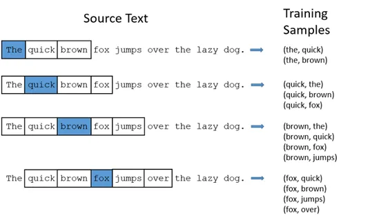
At each step, we pick a target word along with its neighboring context to form a positive training example.

How about the negatives?

If positives are observed from the surrounding context of a target word X, negatives are sampled by throwing in some randomly selected words which we haven’t found appear close to X. This mix challenges the model, teaching it to learn the patterns of words that appear in similar contexts.

Take an e-commerce business as an example. When a user clicks, views, or buys something, that’s a clear positive signal. But what about the millions of items they never touch? Are these items bad, or did the user just never discover them? These are the sorts of “negative” examples—where we assume that most of which he probably won’t pick.

When thinking about the importance of negative sampling, I personally find this analogy helpful: Training a recommendation model without negative samples is like teaching someone to recognize cats by only showing them cat pictures. They might think everything is a cat!

Given that, let’s put some thoughts into different ways we can actually generate negative samples.

Code

All code for this chapter is in notebooks/002-negative-sample.ipynb and src/negative_sampling.py in the project repository.

Negative Sampling Strategies

Random Sampling

Let’s start with the obvious approach: just pick random items the user hasn’t touched.

This is faily straightforward to code up. You grab all the items a user hasn’t interacted with, throw them in a hat, and pull out however many negatives you need. It’s fast, it’s unbiased, and it works.

But there’s a problem. Some of those “random” negatives might actually be items the user would love if they found them. There’s also another issue: the model might get biased toward popular items, since they show up in lots of positive pairs.

Popularity-Based Sampling

To deal with the above popularity bias, instead of picking negatives randomly, we sample them based on how popular they are in the dataset. This makes popular items get chosen as negatives more often.

How does this help? A popular item has a higher chance of being liked by any user than a random item. So when we use popular items as negatives, we’re creating harder training examples. We’re forcing the model to learn why this specific user didn’t interact with this popular item, even though lots of other people did.

The downside? It requires more effort to implement, like tracking popularity statistics when doing sampling. And sometimes it’s true that popular items aren’t always bad choices for a user. They are often top-selling because they’re actually good.

Hard Negative Mining

This is the fancy approach. You need a model that’s already somewhat trained, and you use it to find items it thinks a user would like—but shouldn’t. These become your negative samples.

It’s like having a sparring partner who knows your weaknesses. The model keeps getting challenged by examples that are specifically designed to trip it up. As the model gets better, the negatives get harder, creating a virtuous cycle of improvement.

Sounds great, right? But it’s not always worth the extra effort, especially at the start. You need to train iteratively, which takes more time and compute. And there’s always the risk that you’re just teaching the model to overfit to its own biases.

For this project, we’ll use popularity-based negative sampling. It strikes a good balance between effectiveness and simplicity.

Let’s implement

The full implementation of our negative sampler can be found here.

Function signature:

src/negative_sampling.py

def generate_negative_samples(
    df,
    user_col="user_indice",
    item_col="item_indice", 
    label_col="rating",
    neg_label=0,
    seed=None,
) -> pd.DataFrame:
    """
    Generate negative samples for a user-item interaction DataFrame.
    
    The key insight: sample negative items proportional to their 
    popularity to create more challenging training scenarios.

    Args:
        df (pd.DataFrame): DataFrame containing user-item interactions.
        user_col (str): Column name representing users.
        item_col (str): Column name representing items.
        label_col (str): Column name for the interaction label (e.g., rating).
        neg_label (int): Label to assign to negative samples (default is 0).
        seed (int, optional): Seed for random number generator to ensure reproducibility.

    Returns:
        pd.DataFrame: DataFrame containing generated negative samples.
    """

Let’s walk through each step with both the code implementation and a concrete example to see how popularity-based negative sampling works in practice.

We’ll start with this simple user-item interaction dataset:

Original User-Item Interactions

user_indice	item_indice	rating
1	101	1
1	102	1
2	101	1
2	103	1
2	104	1
3	101	1
3	103	1
4	102	1
4	104	1
5	101	1

Step 1: Calculate Item Popularity

# Calculate item popularity based on interaction frequency
item_popularity = df[item_col].value_counts()

# Convert to sampling probabilities to be used in the next step
popularity = item_popularity.values.astype(np.float64)
total_popularity = popularity.sum()
sampling_probs = popularity / total_popularity

This creates a probability distribution where more popular items have higher chances of being selected as negatives.

Resulting Item Popularity

item_indice	interaction_count	sampling_probability
101	4	0.40
102	2	0.20
103	2	0.20
104	2	0.20

Total interactions: 10, so item 101 (most popular) has 40% sampling probability.

Step 2: Identify Negative Candidates

# Create user-item interaction mapping
user_item_dict = df.groupby(user_col)[item_col].apply(set).to_dict()

# For each user, find items they haven't interacted with
for user, pos_items in user_item_dict.items():
    negative_candidates = all_items_set - pos_items

We make sure we only sample from items the user hasn’t already interacted with.

User’s Positive Items and Negative Candidates

user_indice	positive_items	negative_candidates	num_positives
1	{101, 102}	{103, 104}	2
2	{101, 103, 104}	{102}	3
3	{101, 103}	{102, 104}	2
4	{102, 104}	{101, 103}	2
5	{101}	{102, 103, 104}	1

Step 3: Popularity-Weighted Sampling

# Create a mapping from item to index to quickly access item-related data.
items = item_popularity.index.values
item_to_index = {item: idx for idx, item in enumerate(items)}

# Sample negatives proportional to popularity
candidate_indices = [item_to_index[item] for item in negative_candidates_list]
candidate_probs = sampling_probs[candidate_indices]
candidate_probs /= candidate_probs.sum()  # Normalize

sampled_items = np.random.choice(
    negative_candidates_list, 
    size=num_neg, 
    replace=False, 
    p=candidate_probs
)

This makes sure popular items are more likely to be selected as negatives, creating harder training examples.

For each user, we sample negatives proportional to item popularity among their negative candidates:

User 1’s Negative Sampling

negative_candidate	original_probability	normalized_probability
103	0.20	0.50
104	0.20	0.50

User 4’s Negative Sampling

negative_candidate	original_probability	normalized_probability
101	0.40	0.67
103	0.20	0.33

User 4 will more likely get item 101 as a negative sample since it’s more popular.

In our implementation, we choose to have the same number of negative samples as positive samples. This helps us avoid dealing with imbalanced training data. But feel free to experiment with different ratios (you’ll need to update the implementation).

num_pos = len(pos_items)  # Number of positive interactions
num_neg = min(num_pos, num_neg_candidates)  # Match positive count

Final Result: Complete Dataset

user_indice	item_indice	rating	sample_type
1	101	1	positive
1	102	1	positive
1	103	0	negative
1	104	0	negative
2	101	1	positive
2	103	1	positive
2	104	1	positive
2	102	0	negative
3	101	1	positive
3	103	1	positive
3	102	0	negative
3	104	0	negative
4	102	1	positive
4	104	1	positive
4	101	0	negative
4	103	0	negative
5	101	1	positive
5	103	0	negative

Key Insights:

1. Popularity Bias: Item 101 (most popular) appears more frequently as a negative sample
2. Balanced Sampling: Each user gets the same number of negatives as positives
3. No Self-Contradiction: Users never get negatives for items they already interacted with
4. Harder Training: Popular items as negatives create more challenging learning scenarios

Testing the Implementation

Like other crucial parts of our pipeline, let’s test this with some mock data to make sure it works.

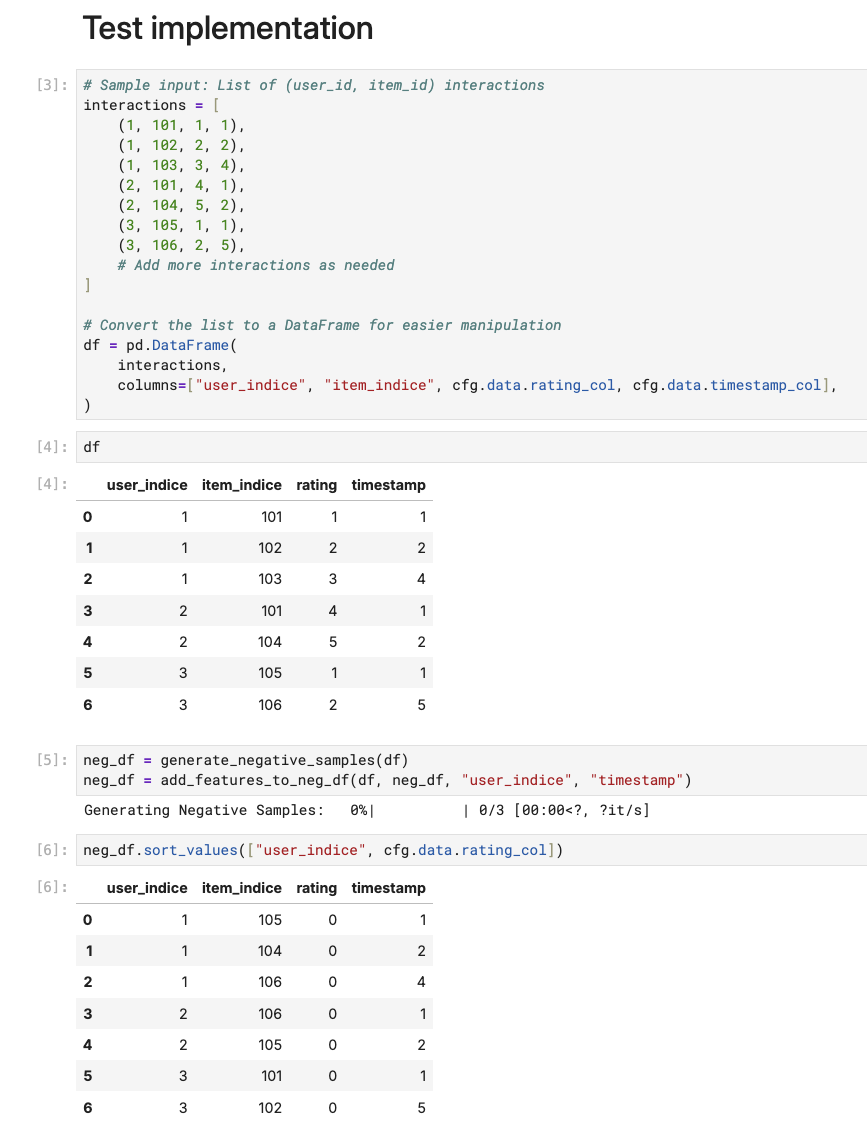
Adding Features to the generated negative samples

As you can see from the above output, we only have the item indice and the label. We also need to populate the new negative samples with the same features as the positive ones, i.e. the sequence of previously interacted items. For this we just need to use the timestamp of the corresponding positive interaction.

def add_features_to_neg_df(pos_df, neg_df, user_col, timestamp_col, feature_cols=[]):
    """
    Add features from positive samples to negative samples DataFrame.
    
    Key insight: Negative samples should have realistic timestamps
    that align with when the user was actually active.
    """
    
    # Create pseudo timestamps for negatives
    # This timestamp pseudo column is used as join key to the positive samples, ensuring that each negative
    # maps to one positive sample and get the positive's features.
    neg_df = neg_df.assign(
        timestamp_pseudo=lambda df: df.groupby(user_col).cumcount() + 1
    )
    
    # Merge with corresponding positive interaction timestamps
    neg_df = pd.merge(
        neg_df,
        pos_df.assign(
            timestamp_pseudo=lambda df: df.groupby([user_col])[timestamp_col].rank(
                method="first"
            )
        )[[user_col, timestamp_col, "timestamp_pseudo", *feature_cols]],
        how="left",
        on=[user_col, "timestamp_pseudo"],
    ).drop(columns=["timestamp_pseudo"])
    
    return neg_df

Concat and re-split train-test

After adding features to the negative samples, we can combine them with the positives. Then we re-split the dataset based on the timestamp milestone we used in our original train-test split.

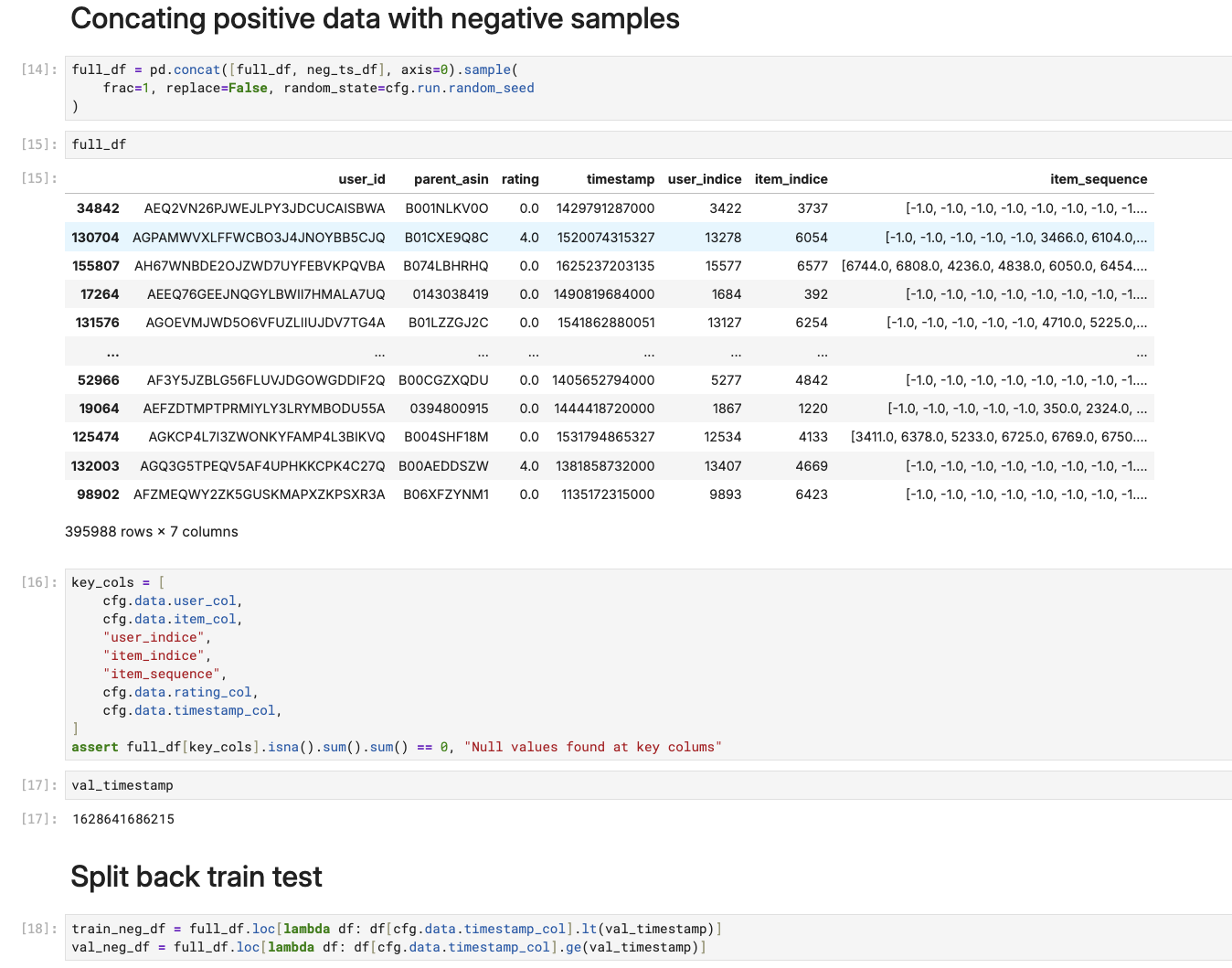
We now have a balanced dataset of positive and negative samples, ready for the next stages in model development cycle!

Recap

In this chapter, we tackled the tricky problem of implicit feedback in recommendation systems. Here’s what we covered:

• Why we need negative samples: Without them, our model would be like someone trying to recognize cats by only seeing cat pictures. We need examples of what users don’t want to create balanced learning.
• Three approaches to negative sampling: We looked at random sampling (simple but not very challenging), popularity-based sampling (our chosen approach that creates harder training scenarios), and hard negative mining (powerful but complex).
• Our popularity-based implementation: We built a system that samples negative items based on their popularity. This forces our model to learn why a user didn’t interact with popular items that others liked.
• Keeping things balanced: We generate equal numbers of positive and negative samples for each user (1:1 ratio) to avoid bias in either direction.
• Adding realistic features: We make sure our negative samples have proper timestamps and features that align with when users were actually active. This maintains temporal consistency for sequence modeling.

Code

All code for this chapter is in notebooks/002-negative-sample.ipynb and src/negative_sampling.py in the project repository.

What’s Next?

We have our labeled data, great. Ready to see some model code?

Not so fast, we will learn about building actual sequence models in … Chapter 5.

In Chapter 4, we’ll set up our evaluation framework and experiment tracking with MLflow while implementing a baseline model along the way as an illustration. This will give us the foundation for systematic model development and comparison.

Continue to the next chapter.

---

If you find this tutorial helpful, please cite this writeup as:

Quy, Dinh. (May 2025). Implement a RecSys, Chapter 3:
Negative Sampling. dvquys.com. https://dvquys.com/projects/implement-recsys/c3/.