Implement a RecSys, Chapter 5: Design Session-based Recommendation System

This is the fifth chapter of the tutorial series: Implement a RecSys.

List of chapters

• Chapter 1: Introduction and Project Overview
  
• Chapter 2: Understanding the Data and Feature Engineering
  
• Chapter 3: Negative Sampling
  
• Chapter 4: Offline Evaluation, MLflow Experiment Tracking, and Baseline Implementation
  
• Chapter 5: Design Session-based Recommendation System
  
• Chapter 6: Preparing for Serving
  
• Chapter 7: Building the API Layer
  

Introduction

In Chapter 4, we established our evaluation framework, implemented MLflow experiment tracking, and built a popularity-based baseline model. Since our baseline is simple, it treats all users similarly—everyone gets the same popular items regardless of their personal browsing history or preferences.

This chapter marks the transition from simple heuristics to a more sophisticated machine learning approach aimed towards personalization. We’ll dive deep into the rationales behind sequence-based recommendation models and explore the design decisions that make them effective.

These models excel at understanding the temporal patterns hidden in user behavior. Instead of just knowing that a user liked certain books, our model will learn to recognize meaningful sequences. For example, when someone browses “Python Programming” followed by “Machine Learning,” the model understands they might be interested in “Deep Learning with PyTorch” next.

This is going to be a long post. So grab your coffee, and let’s dive in.

Code

All code for this chapter is available in the notebooks/011-sequence-modeling.ipynb file and the src/sequence/ directory in the project repository.

Jargon

Throughout the series I would be using sequence modeling and session-based recommendation interchangeably to refer to the same technique of modeling user’s behavior based on their sequential interactions.

Why Sequence Modeling Matters in Recommendations

Traditional collaborative filtering approaches treat user preferences as static snapshots. They might know that User A liked Items 1, 3, and 7, but they miss the story hidden in the order and timing of these interactions.

Consider these two users with identical item preferences but different behavioral patterns:

User A: Book1 → Book2 → Book3 → Book4 → Book5
User B: Book5 → Book1 → Book4 → Book2 → Book3

Both users interacted with the same five books, but their sequences tell very different stories. User A might be following a structured learning path (beginner to advanced), while User B might be jumping between topics based on immediate curiosity. Traditional collaborative filtering would treat these users identically, but sequence models can capture these nuanced patterns.

The even-more-compelling part about this our sequential model is that it gives you two very strong arguments to argue with: real-time adaptation and cold start handling.

Think about what happens in static recommendation systems when new users sign up. They get the same boring popular items everyone else sees. “Here are the top 10 books everyone’s reading!” It’s like walking into a bookstore and having the clerk hand you a list without asking what you’re interested in. The user has to suffer through generic recommendations until the system has enough data about them. This is the cold start problem, which is, trust me, a real typical ask your Product Manager would come up during your recommendation model pitch.

Our sequence model flips this on its head. The moment a new user clicks on their first book, the model springs into action. They browse “Python Programming,” then click on “Machine Learning Basics”—the model immediately understands they’re on a learning journey. The system starts personalizing from interaction number one, like having a shop assistant who gets better at helping you the longer you browse.

And all of this happens without retraining the model or updating any databases as is required from the traditional collaborative filtering approaches, dealing with one of the biggest problems in recommendation systems: how do you stay relevant when user interests change quickly? If thriller readers suddenly start buying romance novels (maybe it’s Valentine’s Day), the model notices the shift in the very next recommendation request.

I hope that now we all understand why sequence modeling is useful. Let’s explore how to actually design it.

Sequence Modeling Approaches

The central challenge in sequence modeling boils down to one question: how do you take a bunch of user interactions and turn them into something expressive for predictions? You have a sequence like “Book A → Book B → Book C” and somehow need to compress all that information into a representation that captures what the user is really interested in.

I like to think of this as a “pooling” problem. You’re pooling information from multiple items into a single representation. It’s like trying to summarize a conversation—you want to keep the important bits and throw away the noise.

The simplest pooling method is averaging. But wait, you might think, average what exactly? We’re talking about sequences of item IDs that users clicked on. You can’t just average “book_123” and “book_456” like they’re numbers, right?

This is where you would want to know about the method of embedding. It converts every item in your catalog into a vector of numbers. Instead of working with raw item IDs, your model works with these dense numerical representations. It’s the same trick that made Word2Vec so powerful—remember from Chapter 3 how it could tell you that “king” minus “man” plus “woman” equals “queen”¹? That magic happens because words become vectors, and vectors can be manipulated mathematically.

So when we talk about averaging a book sequence, we’re actually averaging the its corresponding item embeddings. Both Book A and Book B become 128-dimensional vectors, and averaging them gives you a single 128-dimensional output that somehow captures the essence of “someone who reads both Book A and Book B.”

flowchart TD
    A["User Sequence:<br/>book_123 → book_456 → book_789"] --> B["Item Embedding Layer"]
    
    B --> C["book_123<br/>[0.2, -0.1, 0.8, 0.3, ...]<br/>(128-dimensional vector)"]
    B --> D["book_456<br/>[-0.3, 0.5, 0.1, -0.2, ...]<br/>(128-dimensional vector)"]
    B --> E["book_789<br/>[0.1, 0.3, -0.4, 0.6, ...]<br/>(128-dimensional vector)"]
    
    C --> F["Average Pooling"]
    D --> F
    E --> F
    
    F --> G["Sequence Representation<br/>[-0.03, 0.23, 0.17, 0.23, ...]<br/>(128-dimensional vector)"]

The beautiful thing about embeddings, just like in ML in general, is that they can start random but learn to be meaningful. During training, the model adjusts these vectors so that similar items end up close together in the embedding space. Books about Python programming cluster together, romance novels form their own neighborhood, and so on.

It worths mentioning that averaging² is wonderfully simple, and sometimes simplicity wins. I’ve seen myself trying other pooling methods only to discover that good old averaging works just as well. But that doesn’t mean you shouldn’t experiment. Some sequences have patterns that averaging destroys—like the difference between reading “Beginner Python → Advanced Python” versus “Advanced Python → Beginner Python”.

This is where more sophisticated pooling methods come in. The field of sequence modeling offers several architectural choices, each with its own strengths and trade-offs. The simplest approach uses Recurrent Neural Networks (RNNs), which process sequences step by step, maintaining a hidden state that captures information from previous steps. Think of an RNN as reading a book one page at a time, trying to remember everything important from earlier pages. While this sounds intuitive, vanilla RNNs have a memory problem—they forget important details from way back in the sequence, what researchers call the vanishing gradient problem.

To fix this memory issue, researchers developed Long Short-Term Memory (LSTM) and Gated Recurrent Unit (GRU) networks. These use clever gating mechanisms to decide what to remember and what to forget. GRUs, in particular, have become the go-to choice for recommendation systems. They’re simpler than LSTMs but perform just as well—like getting 90% of the benefit with 60% of the complexity.

More recently, Transformer models have taken the field by storm. Instead of processing sequences step by step, they use self-attention mechanisms to look at all parts of the sequence simultaneously. It’s like being able to read an entire book at once and instantly connect themes from chapter 1 to chapter 20. Transformers are incredibly powerful for capturing long-range dependencies, but there’s a catch—they can be computationally expensive, especially when you have thousands or millions of items in your catalog.

Now that we’ve explored different sequence modeling approaches—from simple averaging to sophisticated Transformers—let’s not forget that all architecture decisions should consider the following question: how do we deploy these models in production systems that need to handle millions of items in real-time?

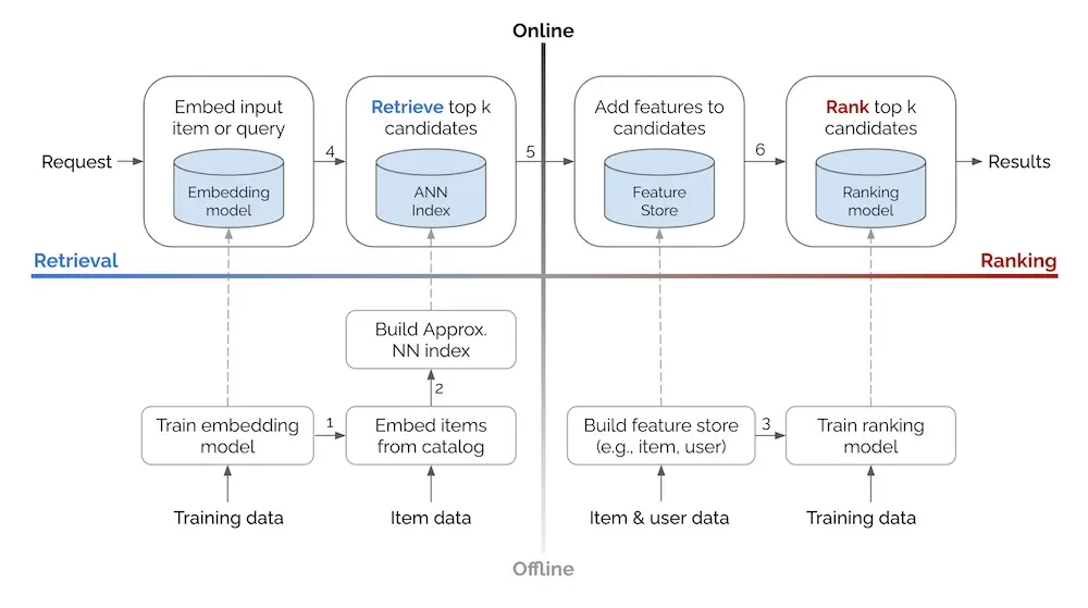
Retrieval vs Ranking

Intuitively, we need to score all items before being able to rank the most relevant and likely-to-be-interacted items on top. But training a scoring model that takes into account each instance of <user, context, item> and serving it for every online request is not feasible because of latency constraints. This act of calculating the scores for millions of items would take forever, and neither our users have that kind of patience nor do we as engineers find that idea sane.

The Two-Phase Architecture

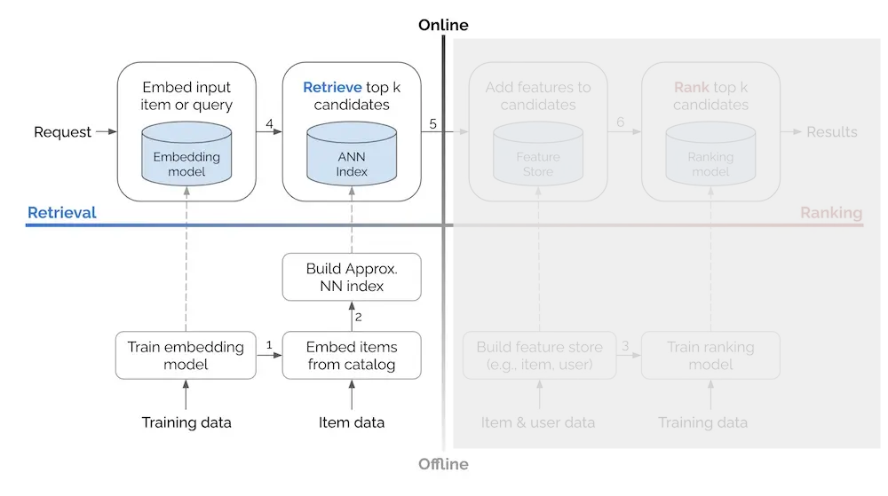
To deal with this problem, we break the whole ranking process into two phases: first we quickly retrieve a candidate shortlist, then we ask a fine-grained ranker to give the final ranking.

The difference in naming between these two phases already reveals their distinct characteristics. The retrieval phase needs to quickly scan millions of items to find about 1,000 potential candidates in milliseconds. This speed requirement means it cannot use complex computations and often needs to leverage indexing structures like vector databases for fast similarity search. The focus here is on recall—ensuring that relevant items make it into the candidate set, even if the initial scoring isn’t perfect.

The ranking phase operates under very different constraints. With bandwidth and a much more limited scope of hundreds to thousands of items, it can afford to adopt many more signals and complex features into its model. This phase delivers much better fine-grained scores for final ordering, focusing on precision—getting the order exactly right among the candidates that have already been deemed potentially relevant.

Yan, Ziyou. (Jun 2021). System Design for Recommendations and Search.

Retrieval as a Standalone System

One important thing to note: apart from returning the candidates, most of the time the retrieval phase can provide scores to indicate how well they match the query. This in fact leads us to an interesting question: Why don’t we just use this signal as a final ranking to show to users?

One obvious argument is that this approach allows us to go to production earlier. Instead of taking months to build a more complete multi-stage system, we get to deploy a working version early, and hence enable early impacts.

More importantly, after the retrieval model is deployed, you start collecting actual interaction data from users engaging with your recommendations. Compare to the historical transaction data, this is a much more valuable feedback to help us further tune the rankings, in both quality and quantity. We have user’s direct feedback to our recommendations by observing which items get clicked/purchased and which ones don’t. And there are just much more data points.

Consider this example of the rich feedback data we can gather:

User-Recommendation interaction logs

rec_id	user_id	timestamp	recommended_items	viewed	clicked	converted
rec_001	user_123	2025-05-31 10:30	[Python_Basics, ML_Intro, Data_Analysis]	Python_Basics, ML_Intro	Python_Basics	Python_Basics
rec_002	user_456	2025-05-31 11:45	[Romance_Novel, Thriller, Biography]	Romance_Novel, Thriller	Romance_Novel	-
rec_004	user_123	2025-05-31 16:00	[Advanced_Python, Deep_Learning, Statistics]	Advanced_Python, Deep_Learning	Advanced_Python, Deep_Learning	Deep_Learning

For user_123, we see a clear learning progression—they converted on both Python_Basics and Deep_Learning, suggesting our sequence modeling is capturing meaningful patterns. User_456 clicked on Romance_Novel but didn’t convert, giving us valuable signal about engagement without satisfaction.

To train a ranking model, we’d explode this data into item-level training examples with binary labels:

Item-level training data for ranking models

rec_id	user_id	timestamp	item	viewed	clicked	converted
rec_001	user_123	2025-05-31 10:30	Python_Basics	1	1	1
rec_001	user_123	2025-05-31 10:30	ML_Intro	1	0	0
rec_001	user_123	2025-05-31 10:30	Data_Analysis	0	0	0
rec_002	user_456	2025-05-31 11:45	Romance_Novel	1	1	0
rec_002	user_456	2025-05-31 11:45	Thriller	1	0	0
rec_002	user_456	2025-05-31 11:45	Biography	0	0	0
rec_004	user_123	2025-05-31 16:00	Advanced_Python	1	1	0
rec_004	user_123	2025-05-31 16:00	Deep_Learning	1	1	1
rec_004	user_123	2025-05-31 16:00	Statistics	0	0	0

Each row represents a <user, context, item> tuple with explicit binary labels. This format captures the full engagement funnel—some items aren’t even viewed (viewed=0), others are seen but not clicked, and a few drive conversions. This multi-level feedback is crucial for training ranking models that understand both what catches users’ attention and what actually satisfies their needs. And the best part is that we don’t have to worry about negative sampling!

Finally, by starting with retrieval alone, we can build our serving and monitoring infrastructure incrementally—learning to handle recommendation traffic, monitor model performance, and debug issues at manageable scale before adding the complexity of a ranking layer.

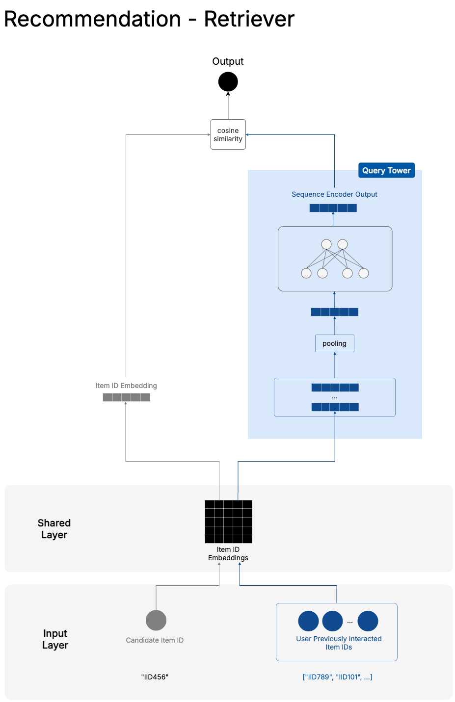
Our Two-Tower Retriever

In that spirit, the implementation of our sequential recommendation model in this series is a retrieval-based one. It follows a typical Two Tower architecture, where the query tower embeds information about the user and context—in our case, the user’s sequence of interactions—while the candidate tower represents the candidate items.

This separation is necessary for efficient serving. The candidate tower can precompute embeddings for all items and store them in a vector index. The query tower only needs to run at request time to generate the user’s current context embedding.

Training Setup

The labels for training come from our preparation in previous chapters. We create positive instances from <user, context, item> tuples which have actual interaction records in the past, while negative examples are sampled from the unseen item space for each user-context pair. This creates a binary classification problem where the model learns to distinguish between items a user would interact with versus items they would ignore.

Serving Architecture

For serving, our retrieval system works in two phases. First, in an offline process, we index all candidate item embeddings in a nearest neighbor vector search system. Then, during online serving, we send the <user, context> as input to the query tower to get a query embedding vector, use similarity lookup to search for the nearest candidate neighbors in the index, and return the corresponding items with their similarity scores.

Retrieval-only system

This architecture enables low-latency response times even when searching through millions of items, making it practical for recommendation serving.

Again, the beauty of this approach is that it’s both a complete recommendation system on its own and a foundation for the more fine-grained ranking models. You can deploy it immediately to start serving personalized recommendations, then later add a ranking layer on top without changing the underlying retrieval infrastructure.

Model Implementation

Now let’s translate the two-tower architecture into concrete code. But first, let me explain a key design decision that shapes our implementation.

The Case for Session-Only Models

Traditional two-tower retrievers include both user embeddings and sequence representations in the query tower. But I’ve chosen to build what I call a “SoleSequenceRetriever”—a model that relies entirely on the sequence of interactions, without any user-specific embeddings.

This isn’t just a technical choice; it’s a strategic one³ that fundamentally changes how the model behaves. By removing user embeddings, we’re making a bet that the sequence itself contains enough signal to make good recommendations. A user browsing “Python Programming → Machine Learning → Data Analysis” tells us more about their immediate intent than knowing they’re “User #47832” with some historical preference profile.

This approach solves several practical problems. New users get meaningful recommendations from their very first interaction—no cold start period where they see generic popular items. Operationally, serving becomes a bit simpler since we don’t need to manage user embedding lookups or worry about user ID mapping issues.

Core Architecture

With that context, let’s look at our implementation.

src/sequence/model.py

class SoleSequenceRetriever(BaseSequenceRetriever):
    def __init__(
        self,
        num_items: int,
        embedding_dim: int,
        pooling_method: str = "mean",
        dropout: float = 0.2,
        mask_pooling: bool = True,
    ):
        self.num_items = num_items
        self.embedding_dim = embedding_dim
        self.pooling_method = pooling_method.lower()
        self.mask_pooling = mask_pooling

        if item_embedding is None:
            self.item_embedding = nn.Embedding(
                num_items + 1,  # extra index for unknown/padding
                embedding_dim,
                padding_idx=num_items,
            )
        else:
            self.item_embedding = item_embedding

        if self.pooling_method == "gru":
            self.gru = nn.GRU(embedding_dim, embedding_dim, batch_first=True)
        elif self.pooling_method == "mean":
            self.gru = None
        else:
            raise ValueError("Invalid pooling_method. Choose 'gru' or 'mean'.")

        self.query_fc = nn.Sequential(
            nn.Linear(embedding_dim, embedding_dim),
            nn.BatchNorm1d(embedding_dim),
            nn.Dropout(dropout),
        )

1

We support pre-trained item embeddings, which can be useful if you have embeddings from other models or external sources.

The architecture reflects our key principles. The item embedding layer converts raw item IDs into dense vectors that can capture semantic relationships. The configurable pooling method (mean or GRU) aggregates the sequence into a single representation. The fully connected layer in the query tower adds learning capacity while batch normalization and dropout help with generalization.

Notice what’s not here: any mention of user IDs. The model’s query tower depends entirely on the sequence of items, making it truly session-based.

Model Training

The forward pass computes cosine similarity between the query embedding (pooled sequence representation) and candidate embedding, scaled to [0,1] to match our binary labels. This choice of cosine similarity isn’t arbitrary—it aligns with how we’ll serve the model using nearest neighbor search in production, i.e. we perform the exact same similarity computation, just against pre-indexed candidate embeddings rather than individual examples.

src/sequence/model.py

class SoleSequenceRetriever(BaseSequenceRetriever):
    # ...

    def get_query_embeddings(self, inputs: Dict[str, torch.Tensor]) -> torch.Tensor:
        item_seq = inputs.get("item_seq")
        if item_seq is None:
            raise ValueError("Missing required input key: 'item_seq'")
        item_seq = self.replace_neg_one_with_padding(item_seq)
        mask = item_seq != self.item_embedding.padding_idx
        seq_embeds = self.item_embedding(item_seq)
        # Pool the sequence; the method will decide whether to use the mask based on self.mask_pooling
        seq_rep = self.pool_sequence(seq_embeds, mask)
        query_embedding = self.query_fc(seq_rep)
        return F.normalize(query_embedding, p=2, dim=1)

    def forward(self, inputs):
        query_embedding = self.get_query_embeddings(inputs)      
        candidate_embedding = self.get_candidate_embeddings(inputs)  
        
        query_embedding = F.normalize(query_embedding, p=2, dim=1)
        candidate_embedding = F.normalize(candidate_embedding, p=2, dim=1)
        cos_sim = torch.sum(query_embedding * candidate_embedding, dim=1)
        
        return (cos_sim + 1) / 2  # Scale to [0,1] since cosine similarity is in [-1, 1]

1

Note how we only need the item_seq from the inputs dict. This handles the cold start problem—new users immediately get meaningful recommendations based solely on their current session, without needing historical preference data.

Mask Pooling

One challenge we need to address: variable sequence lengths. In practice, users have different numbers of interactions—some might have browsed 3 books, others 15. To batch these sequences efficiently for training, we need to pad shorter sequences to a fixed length. We do this by filling empty positions with a special padding token (typically -1).

Masked pooling can help us deal with this issue. Without masking, our pooling operations would include these padding tokens in their calculations, diluting the actual sequence representation. For mean pooling, averaging real embeddings with padding embeddings would give us a less meaningful representation. For GRU pooling, the model might learn spurious patterns from the padding tokens.

By implementing masked pooling, we tell the model to ignore these -1 padding tokens during sequence aggregation. The mask ensures that only genuine user interactions contribute to the final sequence representation, preserving the integrity of the learned patterns.

src/sequence/model.py

class SoleSequenceRetriever(BaseSequenceRetriever):
    # ...

    def pool_sequence(self, seq_embeds: torch.Tensor, mask: torch.Tensor = None) -> torch.Tensor:
        if self.mask_pooling and mask is not None:
            if self.pooling_method == "gru":
                lengths = mask.sum(dim=1).clamp(min=1)
                packed_seq = nn.utils.rnn.pack_padded_sequence(
                    seq_embeds, lengths.cpu(), batch_first=True, enforce_sorted=False
                )
                _, hidden_state = self.gru(packed_seq)
                return hidden_state.squeeze(0)
            elif self.pooling_method == "mean":
                mask_float = mask.unsqueeze(-1).float()
                sum_embeds = (seq_embeds * mask_float).sum(dim=1)
                count = mask_float.sum(dim=1).clamp(min=1)
                return sum_embeds / count

As with other ideas, feel free to experiment with using masked pooling or not. It may sound like a good idea but not always lead to noticeable improvements according to my experience.

Training Loop

The training function uses binary cross-entropy loss against our positive/negative samples. We use PyTorch Lightning to leverage its built-in training loop, logging capabilities and integration with MLflow instead of implementing ourselves⁴.

src/sequence/trainer.py

class LitSequenceRetriever(L.LightningModule):
    # ...

    def training_step(self, batch, batch_idx):
        # Get model's predictions
        predictions = self.model({
            "user_ids": batch["user"],
            "item_seq": batch["item_sequence"], 
            "candidate_items": batch["item"]
        })
        
        # Compare to actual user behavior
        labels = batch["rating"].float()
        loss = nn.BCELoss()(predictions, labels)
        
        # This loss drives the learning process
        return loss

Preparing PyTorch Datasets

PyTorch models work best with PyTorch datasets. Our UserItemRatingDFDataset class handles the conversion from pandas DataFrames to PyTorch tensors:

src/dataset.py

class UserItemRatingDFDataset(Dataset):
    def __init__(self, df, user_col: str, item_col: str, rating_col: str, timestamp_col: str):
        self.df = df.assign(
            **{rating_col: (df[rating_col] / MAX_RATING).astype(np.float32)}  # Normalize rating to [0,1]
        )
    
    def __getitem__(self, idx):
        return dict(
            user=torch.as_tensor(self.df[self.user_col].iloc[idx]),
            item=torch.as_tensor(self.df[self.item_col].iloc[idx]),
            rating=torch.as_tensor(self.df[self.rating_col].iloc[idx]),
            item_sequence=torch.tensor(self.df["item_sequence"].iloc[idx], dtype=torch.long),
        )

This dataset is then wrapped into a PyTorch DataLoader for batching and shuffling.

train_loader = DataLoader(
    train_dataset,
    batch_size=batch_size,
    shuffle=True,
    num_workers=2,
)

Integration with MLflow for Experiment Tracking

Every training run is automatically logged to MLflow through our configuration system:

cfg = ConfigLoader("../cfg/common.yaml")
cfg.run.run_name = "002-sequence-retriever-gru"
cfg.run.experiment_name = "Retrieve - Binary"
cfg.init()  # Automatically sets up MLflow logging

We customzize our Lightning trainer module to help us automatically log:

• Training metrics: Loss, learning rate, weight norms
• Validation metrics: ROC-AUC, PR-AUC, ranking metrics
• Model artifacts: Best model checkpoints

While the model is training, we can observe how it converges and how it performs on the validation set in real-time on MLflow Web UI:

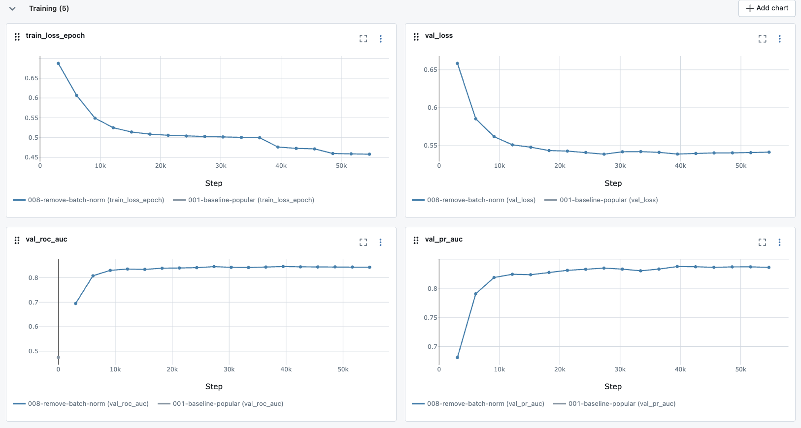
Model Comparison

After training, we can compare the performance of our model with the popularity baseline:

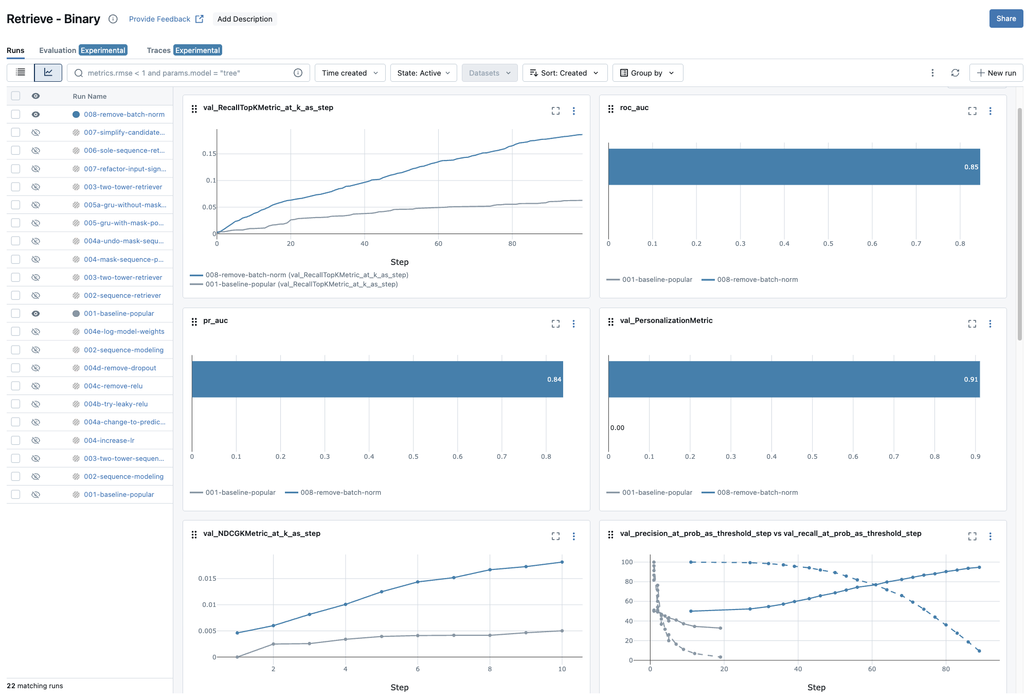
The results validate our sequence-based approach with substantial improvements across all metrics. Let’s break down what these numbers tell us about our retrieval system’s effectiveness.

Recall

Since we’re building a retrieval system, recall is chosen to be our north-star metric. Recall measures what fraction of relevant items we successfully include in our candidate set. In the two-stage retrieval-ranking framework, if our retrieval system misses a relevant item, no amount of sophisticated ranking can fix that—the item is gone forever from the user’s recommendations.

Our sequence-based model achieves significant improvements in recall across thresholds:

• Recall@100: 0.186 vs 0.062 (197% improvement)
• Recall@10: 0.038 vs 0.01 for the popularity baseline (280% improvement)

These numbers tell two important stories. Assuming we would send hundreds of candidates as the output to the later ranking stage, the recall@100 improvement shows we’re nearly doubling our ability to capture relevant items in a typical retrieval pass. This is crucial for the downstream ranking stage—we’re giving it much better raw material to work with.

The recall@10 improvement indicates positive sign but for a different reason. When we deploy this retrieval system as a standalone recommender (without a ranking stage), users see these top-10 results directly. A 280% improvement means users are nearly three times more likely to find something relevant in their immediate recommendations.

Ranking Quality Validation

However, when talking about the end-result ranking for users, NDCG tells a more complete story. The significant improvements in NDCG ranking metrics provide additional validation: NDCG@10: 0.018 vs 0.005 (360% improvement). NDCG measures whether we’re putting the most relevant items at the top of our candidate list. This improvement suggests our retrieval system isn’t just finding relevant items—it’s finding them and scoring them appropriately.

This ranking quality matters regardless of whether we add a downstream ranking stage. If we deploy the retrieval system directly, users get better-ordered recommendations. If we add ranking later, we’re providing the ranking model with better-scored candidates to work with.

What This Means for Users

These metric improvements translate to concrete user experience benefits:

• Immediate Impact: Users are 3x more likely to find relevant items in their top recommendations, dramatically reducing the time spent browsing through irrelevant suggestions.
• Better Cold Start: New users get personalized recommendations from their very first interaction, eliminating the typical cold start period of generic popular items.
• System Flexibility: The improved candidate quality gives us options—we can deploy this as a complete recommendation system now, or use it as a strong foundation for a more sophisticated ranking stage later.

The results demonstrate that sequence modeling captures meaningful patterns in user behavior that static approaches miss entirely.

That said, while the uplifts are strong, the absolute numbers are still low. This is expected since we haven’t really optimized the model, so keep in mind that this is just the beginning. But if you ask me what high or good numbers look like, I would say this kind of improvement is already sufficient for us to deploy in production, given that this is the starting point.

Model Registry and Versioning

As mentioned earlier, MLflow does not only help us track the training process but also provides a model registry for version management and easier deployment. We can easily log the training output artifacts to MLflow, while including a quality gate to ensure that only models that exceed minimum performance thresholds get registered:

# Automatic model registration after successful training
if val_roc_auc > cfg.eval.min_roc_auc:
    # Register model as new version
    mlflow.pytorch.log_model(
        model, 
        cfg.train.retriever.mlf_model_name,
        registered_model_name=cfg.train.retriever.mlf_model_name
    )
    
    # Tag as champion if performance exceeds threshold
    if val_roc_auc > champion_threshold:
        client.set_registered_model_alias(
            cfg.train.retriever.mlf_model_name, 
            "champion", 
            latest_version
        )

1

Champion is a special alias for the current best model. It makes it easier for a new model to go online since we just need to tag it as champion without having to change the code or worry about version number.

That’s it. Finally we are ready to conclude the chapter. If you have made this far, I give you my respect!

Recap

In this chapter, we achieved a major milestone in our recommendation system journey—transitioning from simple heuristic-based approaches to personalized machine learning models that capture temporal patterns in user behavior. Here’s what we accomplished:

From Theory to Practice:

• Why sequence modeling matters: We established that traditional collaborative filtering misses the story hidden in the order and timing of user interactions. By modeling sequences, we can distinguish between users who follow structured learning paths versus those who jump between topics randomly.
• Real-time adaptation and cold start solutions: We demonstrated how sequence-based models solve two critical RecSys challenges. New users get personalized recommendations from their very first interaction, and the model adapts immediately to changing user interests without requiring retraining.

Architectural Decisions:

• Two-tower retrieval architecture: We chose a retrieval-focused approach over end-to-end ranking, enabling fast candidate selection from millions of items while maintaining millisecond-level response times.
• Session-only modeling: By building a “SoleSequenceRetriever” that relies entirely on interaction sequences without user embeddings, we prioritized adaptability and simplified serving infrastructure while solving cold start problems elegantly.

Technical Implementation:

• Masked pooling for variable sequences: We addressed the practical challenge of variable-length user sessions by implementing masked pooling that ignores padding tokens during sequence aggregation.
• Cosine similarity alignment: Our training objective uses the same cosine similarity computation as production serving, ensuring consistency between offline training and online inference.
• PyTorch Lightning integration: We leveraged Lightning’s capabilities for training loops, distributed training, and automatic MLflow integration, avoiding the complexity of custom implementations.

Validation and Results:

• Substantial performance improvements: Our sequence-based retriever achieved 197% improvement in Recall@100 and 280% improvement in Recall@10 compared to the popularity baseline, demonstrating that temporal patterns contain meaningful signals for recommendations.
• MLflow model registry: We established automated model versioning with quality gates, ensuring only models exceeding minimum performance thresholds get registered for potential deployment.

Last but not least, we spent an entire section discussing why whis sequence-based retriever represents a complete, deployable recommendation system that can serve personalized suggestions in real-time. More importantly, it provides a solid foundation for future enhancements—whether adding a downstream ranking layer or incorporating additional features like item content or user demographics.

Code

All code for this chapter is available in the notebooks/011-sequence-modeling.ipynb file and the src/sequence/ directory in the project repository.

What’s Next?

With our sequence-based retrieval model providing significant uplifts compared to the popularity baseline, we have several exciting directions for future development.

Short-term enhancements could include experimenting with adding more input features to our towers, for example:

• Incorporating item content features to improve cold-start item recommendations
• Provide query tower with user profile features, focusing on the information that we may be able to extract even for new users
• Help model be aware of the timings of the items in the interaction sequence

Medium-term evolution might involve building the ranking layer on top of our retrieval system based on the actual feedback labels from the new deployed recommendation module.

Production deployment includes setting up the vector database infrastructure for candidate indexing, implementing real-time serving APIs, and establishing A/B testing frameworks for online evaluation.

In Chapter 6, we will continue our journey to build an end-to-end recommendation system by preparing the offline computation and online serving infrastructure, e.g. MLflow, Redis, Qdrant. The focus would shift a bit towards platform/infrastructure, but we only touch upon how we set them up locally so hopefully it should not be too much of a stretch.

Continue to the next chapter.

---

If you find this tutorial helpful, please cite this writeup as:

Quy, Dinh. (May 2025). Implement a RecSys, Chapter 5:
Design Session-based Recommendation System. dvquys.com. https://dvquys.com/projects/implement-recsys/c5/.

Footnotes

1. If you don’t recall anything about king and queen… Well, yeah, cause I didn’t say anything about that (LOL). But I would assume if you read any random article about Word2Vec, you would run into this famous analogy.

2. Other similarly simple pooling methods are: min, max, sum.

3. Or… it’s not entirely wrong if you think I’m just a lazy guy who doesn’t want to deal with the missing of user embedding for new users 😅.

4. I still remember how frustrating it was trying to implement DDP (Distributed Data Parallel) training loop with pure PyTorch. After figuring out that Lightning does not only handle that elegently but also has a lot of other features that I would have to implement myself, I never looked back.