Implement a RecSys, Chapter 2: Understanding the Data and Feature Engineering

This is the second chapter of the tutorial series: Implement a RecSys.

List of chapters

• Chapter 1: Introduction and Project Overview
  
• Chapter 2: Understanding the Data and Feature Engineering
  
• Chapter 3: Negative Sampling
  
• Chapter 4: Offline Evaluation, MLflow Experiment Tracking, and Baseline Implementation
  
• Chapter 5: Design Session-based Recommendation System
  
• Chapter 6: Preparing for Serving
  
• Chapter 7: Building the API Layer
  

Introduction

In Chapter 1, we set up our development environment and explored the project architecture. Now it’s time to dive into the heart of any recommendation system: data. The quality of our recommendations depends entirely on how well we understand, process, and engineer features from our inputs.

This chapter focuses on the transformation pipeline from raw data to model-ready features. We’ll explore the Amazon Reviews dataset, understand user-item interaction sequences, and build the feature engineering pipeline that powers our session-based recommender.

Code

All code for this chapter is available in the notebooks/000-prep-data.ipynb and notebooks/001-features.ipynb files in the project repository.

Dataset Overview: Amazon Reviews 2023

A good RecSys dataset typically has the following characteristics:

1. Temporal richness: Each interaction has a timestamp, enabling sequence modeling
2. Scale: Millions of interactions across thousands of users and items
3. Real-world patterns: Authentic user behavior with natural sparsity

For this tutorial, instead of using the well-known MovieLens dataset, I chose the Amazon Reviews 2023 collection from the McAuley Lab, specifically the “Books” category. Beyond the above characteristics, it offers other useful signals like user reviews and item descriptions.

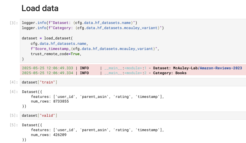
With HuggingFace’s dataset library, we can download everything with just one line of code. The package also caches the downloaded assets by default, so subsequent runs will take almost no time.

from datasets import load_dataset

dataset = load_dataset(
    cfg.data.hf_datasets.name,
    "5core_timestamp_Books",
    trust_remote_code=True,
)

The main schema of the dataset is quite simple:

# From cfg/common.yaml
data:
  user_col: "user_id"
  item_col: "parent_asin"
  rating_col: "rating"
  timestamp_col: "timestamp"

1

Unique user identifier

2

Product identifier (in our case, the ASIN—Amazon Standard Identification Number)

3

User rating (1-5 scale)

4

Interaction timestamp

Configuration Management

from src.cfg import ConfigLoader

# Load configuration
cfg = ConfigLoader("cfg/common.yaml")

Throughout this project, we store most configuration in cfg/common.yaml. This design does not only make it easier for notebooks and scripts to access their inputs and outputs but also help us try different configurations easily.

As you can see above, the train dataset has almost 9M ratings for us to play with. That’s not small at all. However, if you think we’re going to use big data processing for those interactions, this isn’t the case for our series. The first thing I normally do with raw data is to not utilize all the data points.

In fact, I even go the opposite direction.

Data Sampling and Filtering

Let’s discuss why we may consider sampling data as the first thing to do for our project.

If you study the documentation of our Amazon Reviews dataset, you will find that they provide two variants:

Pure IDs (0-Core)

1. Pros of 0-Core: Comprehensive data, Maximum diversity, Rich context, Potential form, Generalization.
2. Cons of 0-Core: Data noise, Large size and high resource demands, Quality variability, Imbalanced distribution.

Pure IDs (5-Core)

1. Pros of 5-Core: Higher quality reviews, Reduced noise, Balanced distribution and Computational efficiency.
2. Cons of 5-Core: Limited diversity, Misalignment with original data distribution, Loss of context, Generalizability and Limited data size for scaling up.

— Amazon Reviews 2023 Dataset Documentation

Pay attention to the pros they give for the 5-Core version: “Higher quality reviews, Reduced noise, Balanced distribution and Computational efficiency”. I find myself specifically resonating with the last aspect.

As ML is mostly about iterative development, it’s by design that the faster we can run operations on our data, the more progress we can make. Being able to quickly experiment different ideas offline offer you a lot of advantages.

For instance, you can rapidly test different feature engineering approaches—whether adding user demographics, item metadata, or temporal features actually improves model performance. You can efficiently compare multiple model architectures (neural collaborative filtering vs. sequential models vs. matrix factorization) within the hours rather than days. Additionally, quick iteration also enables you to discover data quality issues early, such as identifying that certain user segments have vastly different interaction patterns which may suggest a need for new input signals. Finally, fast experimentation saves you a lot of time searching for optimal hyperparameters (learning rates, regularization, etc.).

And after being satisfied with the offline evaluations, we can always commit to train and test the model on the complete dataset.

Given that being said, all sorts of things we want to do to improve our model’s capability can benefit from a small but decent dataset. Obviously the size should not be like a few dozens of observations, cause it hurts with any statistical patterns we would like to learn. In my experience, a good minimum threshold is around 10K users and 5K items, with the sparsity being less than 99.9%.

A note on sparsity

What does it mean to have a decent RecSys dataset? One of the key criteria is sparsity—the ratio of observed interactions to all possible user-item pairs.

To understand why sparsity is problematic, consider the interaction matrix where each cell represents a potential user-item interaction:

	Item 1	Item 2	Item 3	Item 4	Item 5	Item 6
User A	5	-	4	-	-	-
User B	-	3	-	-	5	-
User C	-	-	-	2	-	4
User D	4	-	-	-	-	-

Where numbers represent ratings (1-5) and “-” represents no interaction

In this tiny 4×6 example, only 7 out of 24 possible interactions are observed—giving us 71% sparsity. Real-world recommendation datasets often exceed 99% sparsity.

\[ \text{Sparsity} = 1 - \frac{\text{actual\_interactions}}{\text{num\_users} \times \text{num\_items}} \]

The sparsity problem gets quadratically worse as datasets grow:

Small dataset example: \[\begin{align} \text{users} &= 1,000, \quad \text{items} = 1,000 \\ \text{possible interactions} &= 1,000 \times 1,000 = 1\text{M} \\ \text{actual interactions} &= 50,000 \\ \text{sparsity} &= 1 - \frac{50,000}{1,000,000} = 95\% \end{align}\]

Larger dataset example: \[\begin{align} \text{users} &= 10,000, \quad \text{items} = 10,000 \\ \text{possible interactions} &= 10,000 \times 10,000 = 100\text{M} \\ \text{actual interactions} &= 500,000 \\ \text{sparsity} &= 1 - \frac{500,000}{100,000,000} = 99.5\% \end{align}\]

Each new user adds an entire row of mostly empty interactions, and each new item adds an entire column of mostly empty interactions. Since users typically interact with only a tiny fraction of available items, the interaction matrix becomes increasingly sparse as the catalog grows.

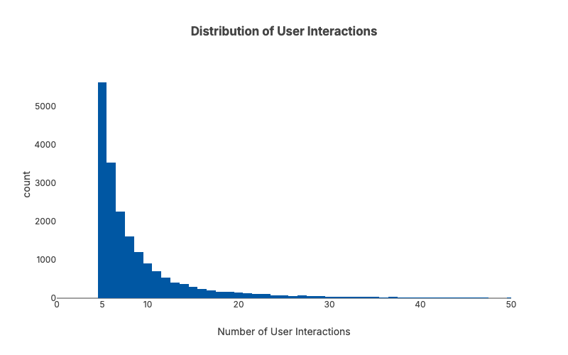
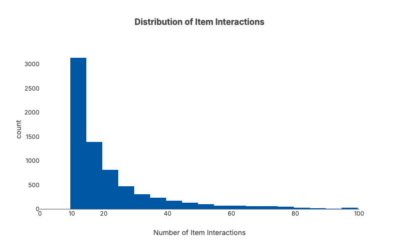
In recommendation systems, interactions follow a long-tailed distribution—many users and items have only a few interactions. So while randomly sampling may work just fine for many ML use cases, we need to apply it a bit more carefully here. Ultimately we want to have a sample dataset where each user/item has at least X interactions.

The tricky part is that a basic random sampling of users and items would create sparsity cascade—a domino effect that breaks your dataset.

Here’s what happens using our 4×6 matrix example: Let’s say User A has 2 interactions (Items 1 and 3), and Item 1 has 2 interactions (from Users A and D). Now suppose we randomly decide to remove User D during sampling. Suddenly Item 1 drops from 2 interactions to just 1 interaction from User A. If our minimum threshold is 2 interactions per item, Item 1 now becomes too sparse and gets removed. But removing Item 1 means User A loses one of their interactions and might fall below the minimum user interaction threshold as well.

Original Matrix

	Item 1	Item 2	Item 3	Item 4	Item 5	Item 6
User A	5	-	4	-	-	-
User B	-	3	-	-	5	-
User C	-	-	-	2	-	4
User D	4	-	-	-	-	-

Item 1 has 2 interactions (Users A, D) ✓

Remove User D

	Item 1	Item 2	Item 3	Item 4	Item 5	Item 6
User A	5	-	4	-	-	-
User B	-	3	-	-	5	-
User C	-	-	-	2	-	4
User D	4	-	-	-	-	-

Item 1 now has only 1 interaction (User A) ✗ - Below threshold!

Remove Item 1 (below threshold)

	Item 1	Item 2	Item 3	Item 4	Item 5	Item 6
User A	5	-	4	-	-	-
User B	-	3	-	-	5	-
User C	-	-	-	2	-	4

User A now has only 1 interaction (Item 3) ✗ - Might fall below user threshold too!

It’s like pulling threads from a sweater—everything starts unraveling.

An iterative approach can be considered to deal with this kind of problem. We gradually drop random users from the dataset while watching our conditions and sampling targets. The trade-off is that while it’s hard to get an exact predefined number of users and items, we can control the minimum acceptable thresholds:

cfg/common.yaml

sample:
  sample_users: 10000
  min_val_records: 5000
  min_user_interactions: 5
  min_item_interactions: 10

1

We need to ensure sufficient validation data to evaluate our models.

from src.sample import InteractionDataSampler

data_sampler = InteractionDataSampler(
    user_col=cfg.data.user_col,
    item_col=cfg.data.item_col,
    sample_users=cfg.sample.sample_users,
    min_val_records=cfg.sample.min_val_records,
    random_seed=cfg.run.random_seed,
    min_item_interactions=cfg.sample.min_item_interactions,
    min_user_interactions=cfg.sample.min_user_interactions,
    perc_users_removed_each_round=0.1,
    debug=False,
)

...

Randomly removing 2960 users - Round 18 started
After randomly removing users - round 18: num_users=29,605
Number of users 29,605 are still greater than expected, keep removing...

Randomly removing 2413 users - Round 19 started
After randomly removing users - round 19: num_users=24,137
Number of users 24,137 are still greater than expected, keep removing...
Number of val_df records 4,282 are falling below expected threshold, stop and use `sample_df` as final output...

len(sample_users)=19,734 len(sample_items)=7,388

InteractionDataSampler implementation

After sampling, we end up with 19,734 users and 7,388 items. The sample dataset has 99.8666% sparsity compared to 99.9976% sparsity from the original dataset.

Train-Test Split

To evaluate our models, we need to split it into a train and validation dataset. The validation dataset plays a critical role in providing an estimate of how well the model performs on unseen data.

There are two main types of train-test-split in RecSys:

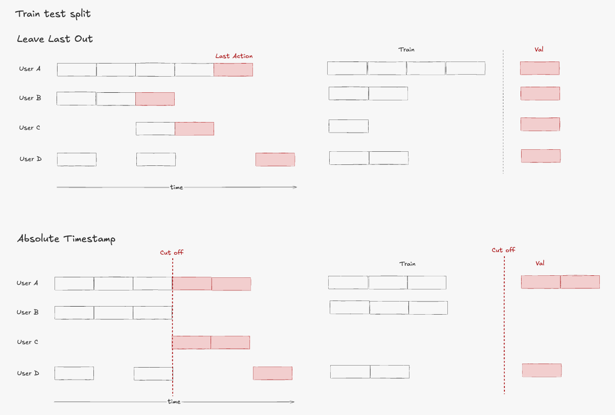
From what I’ve seen, last-one-out is used more in academic settings, while absolute timestamp is more common in industry. This makes sense from the perspective that any model deployed in production gets tested against future data.

Feature Engineering

ID Mapping: From Strings to Indices

As discussed in Chapter 1, we’re modeling this problem with neural networks. Deep learning models work with numerical indices, not string IDs. So we use our IDMapper to provide deterministic mapping from user and item IDs to integer indices:

from src.id_mapper import IDMapper

user_ids = train_df[cfg.data.user_col].values
item_ids = train_df[cfg.data.item_col].values
unique_user_ids = list(set(user_ids))
unique_item_ids = list(set(item_ids))
idm = IDMapper()
idm.fit(unique_user_ids, unique_item_ids)

# Save for later use in model serving
idm.save("data/idm.json")

# Below is the example output of the indice mapping for user IDs:
display(idm.user_to_index)

{
  "AE224PFXAEAT66IXX43GRJSWHXCA": 0,
  "AE225Y3KDZ44DHLUKLE4RJ63HC5Q": 1,
  "AE226YVDC3MAGJZMZ4IBGE7RFJSQ": 2,
  "AE22EJZ4354VB7MN4IE2CDGHA2DQ": 3,
  "AE22O3TURLPFCJKL7YCX5CPF22OA": 4
}

Sequence Generation

After nearly two chapters, you might probably wonder about the term “sequence” I keep mentioning over and over, yet still missing an explanation. How does user-item rating data relate to sequences?

Traditional collaborative filtering approaches like Matrix Factorization only use the user-item rating matrix. But one important signal gets left out: the timestamps.

The key insight is simple: when a user interacts with items over time, those interactions tell a story. We group each user’s interactions chronologically to create sequences of items, with the assumption that items a user engages with have meaningful relationships to each other.

Let’s trace through an example to understand how sequence generation works.

Suppose we have the following user interactions over time:

Time	Item Purchased	Item Index
1	Python Programming	42
2	Machine Learning	73
3	Deep Learning	91

This is the expected output in terms of the user-item sequence signals:

Row	Target Item	Item Sequence	Previous Items
1	42 (Python Programming)	[-1, -1, ..., -1]	No previous items
2	73 (Machine Learning)	[-1, -1, ..., 42]	Python book
3	91 (Deep Learning)	[-1, -1, ..., 42, 73]	Python, ML books

The function generate_item_sequences can be used to perform the sequence generation.

from src.sequence.util import generate_item_sequences

# Sample DataFrame
data = {
    "user_indices": [0, 0, 1, 1, 1],
    "item_indices": [0, 1, 2, 3, 4],
    "timestamp": [0, 1, 2, 3, 4],
    "ratings": [1, 4, 5, 3, 2],
}

df = pd.DataFrame(data)

# Generate the item sequences
df_with_sequences = generate_item_sequences(
    df,
    user_col="user_indices",
    item_col="item_indices",
    timestamp_col="timestamp",
    sequence_length=3,
    padding=True,
    padding_value=-1,
)

display(df_with_sequences)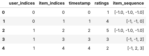

As you can see, the above item_sequence column contains the sequence of items in chronological order which holds the context for the model to understand user preferences and make sequential predictions.

In this project, we use the user’s last 10 items as the sequence length, but this is configurable. The choice depends on experimentation, but generally there’s a trade-off: longer sequences provide more context but use more memory, while shorter sequences focus on recent items and process faster.

cfg/common.yaml

train:
  sequence:
    sequence_length: 10  # Keep last 10 items as context

Do take note that we need to pad sequences to the same length so we can batch process them in our PyTorch model.

With our feature engineering pipeline complete, we now have transformed our raw Amazon Reviews data into model-ready sequences. Each user’s interaction history has been converted into numerical sequences that capture temporal patterns, while our ID mapping ensures consistent encoding across train and validation sets. These sequences will serve as the foundation for training our neural sequential recommendation model, providing the rich contextual information needed to predict what items users are likely to engage with next.

Recap

In this chapter, we have covered:

1. Data Sampling and Filtering: We discussed problems with basic random sampling of dyadic data and introduced our iterative sampling approach
2. ID Mapping: We converted string IDs to numerical indices to work with PyTorch model
3. Sequence Generation: We created item sequence features based on user’s chronological interactions

Code

All code for this chapter is available in the notebooks/000-prep-data.ipynb and notebooks/001-features.ipynb files in the project repository.

What’s Next

In Chapter 3, we’ll tackle the critical challenge of negative sampling. If our model only sees positive interactions (ratings), it can’t learn meaningful patterns for generalization. We need to generate negative examples so the model can distill the patterns by learning to distinguish between positive and negative interactions.

Continue to the next chapter.

---

If you find this tutorial helpful, please cite this writeup as:

Quy, Dinh. (May 2025). Implement a RecSys, Chapter 2:
Understanding the Data and Feature Engineering. dvquys.com. https://dvquys.com/projects/implement-recsys/c2/.